Market Makers in Decentralized Exchanges
Last Updated on 3. May 2023 by Martin Schuster
Order books work best in vibrant markets with frequent trades. But not every market is like that. In order to facilitate a good trading experience, a market maker can come into play. A market maker immediately buys and sells orders independently if there is a matching buyer or seller. Thus, they provide liquidity.
Typically, market makers make a profit by buying at a lower price than they anticipate to sell for. An example is to buy 100 tokens for 100 coins and sell them for 100.5 coins. The difference is the bid-ask spread.
A market maker that works like that faces a loss risk. To reduce this risk, it needs good information about the market and has to anticipate the price development, demand, and supply. If, for example, the quoted bid price (sell) is too low, the market maker runs out of tokens (or stocks). If the asked price (buy) is too high, the market maker will run out of funds. This makes it difficult to use in a decentralized setup.
But there are other designs of market makers that allow a less risky operation. Here, the market price is calculated with a curve.
Pricing Curves
Pricing curves are a way to automate a market maker. They allow a continuous buy and sell offer. If a trader arrives, it will always find an offer. And if he is willing to pay the proposed price, the trade will take place. In this topic, you learn how pricing curves work and what their advantages and disadvantages are.
In order to work, these exchanges need a liquidity pool for each trading pair. Typically, everybody can provide some liquidity to the so-called liquidity pools. Liquidity providers are rewarded with fees.
You can find an overview and analysis of exchanges with automated market makers here.
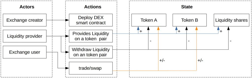
The following figure shows the tasks of each actor: exchange creator, liquidity provicer, and exchange user.
Constant Product Function
The simplest pricing curve is the so-called constant product function (CPF). It looks like this:
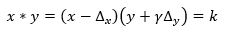
Where:
x: amount of token X in the liquidity pool
y: amount of token Y in the liquidity pool
k: constant number (=product of the formula)
dx/y: Change of the token’s amount
This means that the product k of x and y must always remain the same with every trade. The less of token x is in the pool, the more expensive it gets in terms of token y. The slope of the function gives the exchange ratio (price) at a certain point.
We call this price spot price. It tells us how much a very tiny amount of token A costs in terms of token B.
The following chart shows the relations.

Example 1
Let’s assume we have the following liquidity pool:
- amount token A: 50
- amount token B: 100
- k = 5000
The slope pA = 100/50 = 2
This means that a trader who wants to buy a tiny amount of token A has to pay 2 token B.
But if the buyer buys a certain amount of token A, we have to change the position on our curve. And different positions on the curve mean different slopes. This is called price slippage.
Price Slippage
Example 1
In the following example, we show how to calculate the price. In our liquidity pool, we have tokens A and B.
- amount token A: 50
- amount token B: 100
- k = 50 * 100 = 5000
If we want to buy one token A, this reduces its amount to 49 (50-1=49). To maintain k=100, we need to calculate the new amount of token B by 5000/49 = 102.0408. After the trade, we would need to have 49 token A and 102.0408 token B in our liquidity pool.
So, for one token A our buyer has to pay 2.0408 token B. This is more than the spot price (slope) of 2.
Example 2
In our second example, we have a liquidity pool with:
- amount token A: 10
- amount token B: 500
- k = 10*500=5000
Token A is compared to the first example much scarcer. Again, we want to calculate the price for one token A.
To maintain k = 5000, our buyer has to pay 5000/9=555.5556 tokens B. If we compare this to the first example, we see that it got much more expensive to buy the same amount of a token if it becomes scarce.
This increasing price ensures that the liquidity pool is never empty. The following diagram shows the slope of the price depending on the amount of token A available in the liquidity pool. The steeper the slope is, the more expensive is it to buy the token.

Price Slippage
Create new Liquidity Pool
Curve’s Function
Slippage can be a problem since large amounts of liquidity are necessary to avoid price changes during a trade. This makes it less liquidity efficient.
A pricing formula without slippage would be a constant sum (not constant product) function. Here, the total number of all tokens in a liquidity poll remains constant. If you remove an amount x of one token, you need to supply the same amount of the other token. The ratio is always 1, which means that there is no slippage. The problem, however, is that the price never changes and thus cannot adapt to the market price. As a result, arbitrage traders could empty the liquidity pool by buying the underpriced token.
A solution could be to combine the constant product formula with the constant sum formula so that the slippage is low around the most important price (exchange ratio).

The yellow line represents the constant sum function and the dashed line the constant product function. The bold black line is a combination of both constant sum and constant product function. The slippage is low around the balance spot, but it increases rapidly if the difference to this spot becomes too big. Curve introduced the following formula:
n: Number of different tokens in the Liquidity pool: If the liquidity pool contains, for example, ETH and DAI n = 2
D: Amount of tokens: If there are 100 ETH and 100 DAI in the pool, D = 200
xi: Amount of token i
A: A constant where the portfolio is in balance
When adding a token xi, the equation must remain true. This can be done by an iterative process for finding D or xj.
This type of function is useful for assets that revolve around an optimal ratio (price) like stable coins. The exchange creator has to choose the constant A carefully that the low slippage area covers this spot. If the price permanently shifts way from the optimal spot, the slippage is even higher than the constant product function.

 Register
 Sign in