Mixed Strategies

So far, we have only considered pure strategies. But if we repeat a game, we can change the strategy in every round. This is called a mixed strategy. The strategy is, in this case, the probability of choosing a certain (pure) strategy.

Let’s consider the following example:

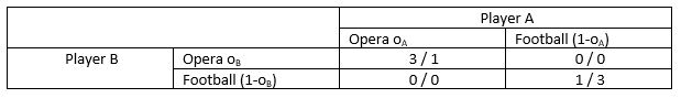
We can see that there are two Nash equilibria in pure strategies {Opera; Opera} and {Football; Football}.

But if this game is repeated, both participants could randomize their decision with a probability 0 of going to the opera. 1-0 would then be the probability of going to football.

The question is, what is the optimal mixing probability?

Calculation of Equilibria in Mixed Strategies

First, we need to find the equation for the expected value. We multiply the probabilities of each strategy combination

For player A this is:

E_A = 1 * o_A * o_B + 0*o_A * (1-o_B) + 0 * (1-o_A) * o_B + 3 * (1-o_A) * (1-o_B)

For player B we have:

E_B = 3 * o_A * o_B + 0*o_A * (1-o_B) + 0 * (1-o_A) * o_B + 1 * (1-o_A) * (1-o_B)

For player A we get

E_A = 1 * o_A * o_B +  3 * (1-o_A) * (1-o_B)

E_A = 4 * o_A * o_B  +  3 -3o_A  -3o_B

Calculating the maximum via the first derivative:

dE_A/do_A = 4o_B – 3 = 0

o_B = 0.75

For player B we get:

o_A = 0.25

We see that each player depends on the probability that his opponent chooses. So, we get the highest expected value if player B chooses opera with a probability of ¾ and B chooses football with the probability of ¼.

The expected value for A is: 0.75

The expected value for B is: 0.75

Simplification of the Equation

To calculate the equilibrium in mixed strategies, one always needs to conduct the same steps.

• Set up an equation for the expected value
• Calculate the first derivative
• Set first derivative zero and solve it

If we want to do this repeatedly, this becomes pretty time-consuming. For that reason, we can calculate the final equation with parameters and fill them in accordance with the pay-off matrix later.

The following pay-off matrix contains parameters instead of numerical values. Upper case letters are the pay-offs for player B and, lower case letters belong to player A.

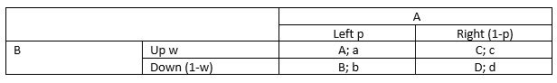
E_A = apw + bp(1-w) + c(1-p) + c(1-p)w + d(1 – p)(1 – w)

dE_A/dp = aw + b – bw – cw -d + dw = 0

As a formula for w we get:

w =(b-d)/(-a+b+c-d)

We do the same for player B and get:

p = (C-D)/(-A+B+C-D)

These equations make it easier for us to calculate the equilibrium in mixed strategies.

Limitations of Equilibria in Mixed Strategies – No Maximum

While mixed strategies can help us solve a coordination game, they don’t necessarily give us the best result.

One issue can be that there is no maximum.

Let’s consider the following example.

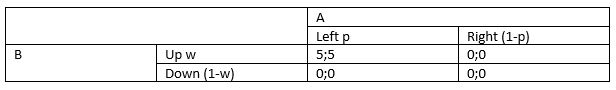
The equilibrium in mixed strategies would be:

p = 0

w = 0

It would tell us always to play right and down. However, this doesn’t make sense since we would receive zero pay-offs. The efficient Nash equilibrium is {left, up}.

The reason is that the second derivation is not < zero, which means that we didn’t calculate the maximum.

Limitations of Equilibria in Mixed Strategies – No Stable Equilibrium

A Nash equilibrium is defined as a strategy combination where no participant wants to change its decision unilaterally. That is because this participant would be worse off than before changing his mind.

In an equilibrium in mixed strategies, this is not necessarily the case. As we saw, the maximum of the expected value depends not on your own probability but on the probability of the other player.

Let’s consider the following numerical example:

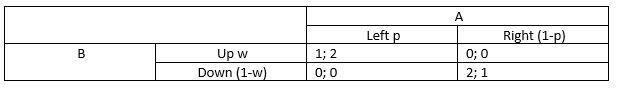
Our equilibrium in mixed strategies would be:

p = 2/3

w = 1/3

We can calculate the expected values for every probability combination. Given that player B choses Up with w = 1/3

p	0.00	0.10	0.20	0.30	0.40	0.50	0.60	2/3	0.7	0.80	0.90	1.00
B	1.33	1.23	1.13	1.00	0.93	0.83	0.73	0.67	0.63	0.53	0.43	0.33
A	0.67	0.67	0.67	0.67	0.67	0.67	0.67	0.67	0.67	0.67	0.67	0.67

We can see that if p changes (the probability of A to play Left), the expected pay-off for A remains the same (=0.67). It only affects the pay-offs for B.

B can notice this deviation from the originally expected pay-off and adjust his w accordingly. This would cause a change in A’s pay-offs. He could then adjust his p.

Interestingly, this adjustment doesn’t necessarily lead to the equilibrium in mixed strategies. It can lead to an equilibrium in pure strategies. Hence, an equilibrium in mixed strategies is not necessarily stable.

Limitations of Equilibria in Mixed Strategies – Randomness

To play an equilibrium in mixed strategies, both players need a good source of randomness. This is hard to achieve. It is also hard to observe if one player really plays randomly. Only with large datasets deviations from the equilibrium are detectable.