Confusion Matrix

Last Updated on 27. September 2024 by Mario Oettler

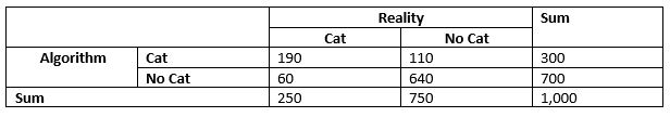
Suppose we have an algorithm that recognizes cats in photos. Our data set consists of 1,000 photos. 250 show a cat, and the rest doesn’t. Our algorithm classifies 300 photos as a picture of a cat. Of these photos, 190 are correctly classified.

What is the likelihood that a photo classified by our algorithm as a “cat photo” really shows a cat?

Example 1

We can create a matrix that lists all possible results for that purpose.

Here are some hints on how to fill the matrix.

• As we said, we have 250 pictures with a cat. 190 of them are correctly recognized by our algorithm. This leaves 60 photos that were incorrectly classified as “No Cat”.
• We also know that our algorithm found 300 photos were it thought they show a cat. Since only 190 were correct, 110 are no cat in reality.
• In total, we have 1,000 photos, which means that 1,000-250 = 750 photos don’t show a cat in reality.
• With this information, we can calculate the number of photos that our algorithm correctly classified as “No Cat”.

To answer our question, what is the likelihood that a photo classified as “Cat” by our algorithm shows a cat in reality, we calculate:

190/300 = 63.33%

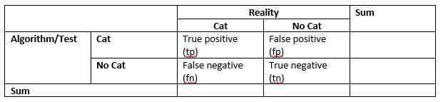
This confusion matrix helps us to assess the quality of an algorithm or test.

The fields in the matrix give us the following information:

Example 2

Let’s consider another example.

Suppose our algorithm classifies every photo as “Cat”. What would the confusion matrix look like?

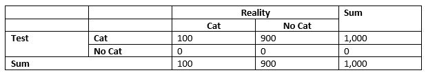
What is the likelihood of getting a cat photo if the test shows “cat”?

1,000/100 = 0.1

Example 3

Now, our test randomly displays “Cat” or “No Cat” (50:50). The confusion matrix would look like:

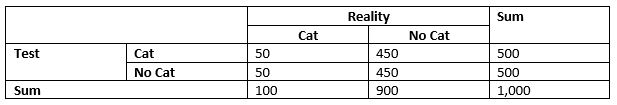
What is the likelihood of getting a cat photo if the test shows “Cat”?

50/500 = 0.1

As you see, two different tests bring the same likelihood. Hence, in order to assess the quality of the algorithm (or test), we need to calculate some indicators:

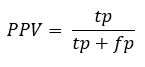
Precision or Positive Prediction Value (PPV)

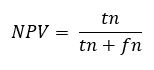
Negative Prediction Value (NPV)

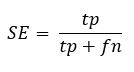
Sensitivity (SE) or true positive rate (TPR)

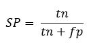
Specificity (SP) or true negative rate (TNR)

KPI	Example 1	Example 2	Example 3
Precision or Positive Prediction Value (PPV)	0.633	0.1	0.1
Negative Prediction Value (NPV)	0.914	DIV/0!	0.9
Sensitivity (SE)	0.76	1	0.5
Specificity (SP)	0.85	0	0.5

The PPV (Positive Prediction Value) and NPV (Negative Prediction Value) can only be applied to other groups (or data sets) if the pre-test probability (prevalence) is the same in both groups.

To make up for this limitation, one can calculate the likelihood ratio:

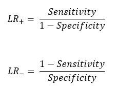
Likelihood ratios compare the probability that someone with the disease, or in our case a picture with a cat, has a particular test result as compared to someone without the disease or a picture without a cat.

They exist for a positive test result and for a negative test result.

The positive likelihood ratio (LR₊) tells us how the likelihood of a positive result changes if the test result is positive (or the algorithm says “Cat”).

The negative likelihood ratio (LR_–) tells us how the likelihood of a positive result changes if the test result is negative (or the algorithm says “No cat”).

A likelihood ratio of 1.0 indicates that there is no difference in the probability of the particular test result (positive result for LR+ and negative result for LR−) between those with and without the tested feature (cat).

A likelihood ratio >1.0 indicates that the particular test result is more likely to occur in pictures with a cat than in those without a cat.

A likelihood ratio <1.0 indicates that the particular test result is less likely to occur in those pictures with a cat those without a cat.

The greater the distance of the LR from 1, the greater the significance of the test.